Time Series Analysis in Python

What Is Time Series Analysis?

Time series analysis consists of statistical and machine learning techniques that allow you to extract meaningful information from data collected over time. Analysis may include methods for extracting trends and seasonal elements from historical data, as well as forecasting future values.

Why Use Python for Time Series Analysis?

There are numerous programming languages you can choose from to analyze time series data. However, Python dominates the data science industry due to its simplicity, versatility, and, most importantly, powerful features. You will learn different techniques and methods that will allow you to easily work with time series data using Python.

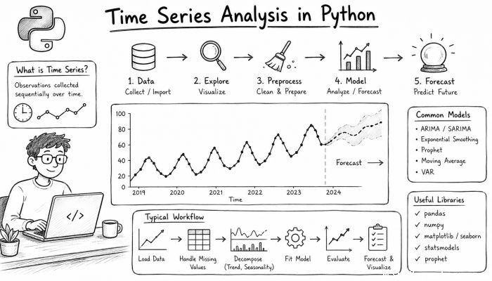
Table of Contents

- Understanding Time Series Data 

- Setting Up the Python Environment 

- Importing and Preprocessing Data 

- Visualizing Time Series Data 

- Stationarity and Why You Should Care About It

- Autocorrelation and Partial Autocorrelation Plots 

- Classical Time Series Modeling: AR, MA, ARMA, and ARIMA

- Seasonal Time Series Models: SARIMA and Seasonal Decomposition

- Facebook's Prophet Library for Easy Forecasting 

- Machine Learning for Time Series Forecasting in Python

- Model Validation and Evaluation 

- Time Series Analysis Applications 

- Wrap-up 

Understanding Time Series Data

Time series data — also known as a temporal data set — consists of values obtained through observations made at regular time intervals (e.g., minute, hour, day). Since time series data is dependent on time (past values affect future values), it differs from the data that you might analyze to answer classification or regression problems.

Characteristics of Time Series Data

- Trend — Time series data usually has an underlying trend. The trend shows the general direction in which the data is moving.

- Seasonality — Seasonal effects exist when your data is affected by seasonal factors, such as day of the week, month, quarter, etc.

- Cyclicity — Cyclical data refers to fluctuations happening at inconsistent time intervals.

- Noise — Noise is undesirable random variations that usually exist within time series data.

Preprocessing Steps for Time Series Data

When working with time series data there are certain things you should keep in mind during the preprocessing stage. Depending on the data you are working with you might have to do some of (or all) of the following.

- Handling missing data. 

- Filtering out noise. 

- Convert data to different time zone. 

- Resampling data to change the frequency. 

Typically you will not have to do much feature engineering when working with time series data as the variables you are analyzing will most likely be your features.

Setting Up the Python Environment

Python offers many libraries that you can use to work with time series data.

Libraries you may use to work with time series data

- pandas.DatetimeIndex — Helpful when dealing with time series data.

- matplotlib.pyplot — Allows you to visualize your data. 

- statsmodels.api, sklearn — Used for modeling your data. 

- prophet — Library developed by Facebook for forecasting. 

To set up your Python environment for time series analysis you will first have to install the packages you intend to use. We recommend using either pip or conda to manage your package installations.

Importing and Preprocessing Data

As with most projects, you will first have to load your data. You can import CSV, Excel files, or pull data directly from a database.

Loading Data Tips 

- Make sure to set parse_dates=True when reading CSV files so that pandas will treat the dates as a DatetimeIndex.

- Consider converting the time series to a different time zone using data_obj.tz_convert(timezone).

- If needed, change the frequency of your data using data_obj.resample(rule).

Missing Values 

If your dataset contains any missing values you can fill them in using pandas.fillna() method or you can interpolate the missing values using pandas.interpolate().

Visualizing Time Series to Detect Patterns

Visualizing your data can help you identify obvious patterns, trends, and outliers. You should take the time to plot your data as it will allow you to better understand the data you are working with.

Time Series Plot

You should first plot the time series. You can do this by passing your dates on the x-axis and the data you wish to plot on the y-axis.

Rolling Mean 

You can apply rolling statistics to smooth out short term fluctuations and highlight long term trends in the data.

Decomposition Plot 

You can decompose your time series data into three categories: trend, seasonality, and residuals.

Autocorrelation Plot (ACF)

You can use statistical plots such as autocorrelation plots to check for lag correlations.

Stationarity and Why You Should Care About It

Testing and achieving stationarity is an important step when analyzing time series data. A time series dataset is said to be stationary if the mean, variance, and covariance of the data remain constant over time.

Stationarity Check Plots

You can check if your data is stationary by simply plotting it. You should look out for changing mean and variance over time.

Statistical Tests for Stationarity

There are several statistical tests you can use to check for stationarity. Two of the most commonly used tests are:

- KPSS Test: To check stationarity 

- ADF Test: To check for non-stationarity 

If your data is not stationary there are certain transformations you can apply to stabilize the mean and variance. Common transformations include difference and log transformations. 

Autocorrelation and Partial Autocorrelation

Autocorrelation is the correlation of a signal with a delayed copy of itself. As mentioned earlier, you can use statistical plots to check for autocorrelation.

Autocorrelation Function (ACF) Plot 

An autocorrelation plot can help you identify whether any lag values are significantly different from others.

Partial Autocorrelation Function (PACF) Plot 

The partial autocorrelation plot is used to spot significant lag values. A significant lag could help you determine the order of an AR or ARMA model.

--- 

Classical Time Series Modeling: AR, MA, ARMA, and ARIMA

Classical time series models include Auto-Regressive (AR) models, Moving Average (MA) models, Autoregressive Moving Average (ARMA), and Autoregressive Integrated Moving Average (ARIMA) models.

Auto-Regressive Models: AR(p)

Auto-Regressive models use dependency between an observation and its lagged values to predict future values.

Moving Average Models: MA(q)

Moving Average models use dependency between an observation and a residual error from a moving average model applied to lagged observations.

Autoregressive Moving Average Models

ARMA(p,q) 

Autoregressive Integrated Moving Average Models:

ARIMA(p,d,q) 

Seasonal Time Series Models: SARIMA and Seasonal Decomposition

Seasonal ARIMA, or SARIMA, is an extension of ARIMA that supports univariate time series data with seasonality.

Seasonal Decomposition of Time Series (STL) 

Facebook's Prophet Library for Easy Forecasting Machine Learning for Time Series Forecasting in Python

As machine learning has gained more traction, we have seen many algorithms arise that can be used to forecast time series data.

Model Evaluation 

Time Series Analysis Applications

Knowing how to analyze time series data can allow you to apply these skills to a wide range of problems.

- Anomaly detection on sensor readings. 

- Hospital bed management by predicting patient admissions. 

- Stock price forecasting. 

- Predicting customer retention and churn. 

- Predicting energy demands. 

Wrap-up

Congratulations on making it to the end of the tutorial. I hope you learned something new and will be able to apply your newly found skills to your everyday data analysis tasks. If you have any questions, feel free to reach out to me on Twitter at [@RaRe-Technologies](https://twitter.com/RaRe-Technologies). Happy forecasting!